RESEARCH/REVIEW ARTICLE
Automated ice-sheet snowmelt detection using microwave radiometer measurements
Lei Liang,1 Huadong Guo,1 Xinwu Li1 & Xiao Cheng2
1 Key Laboratory of Digital Earth, Institute of Remote Sensing & Digital Earth, Chinese Academy of Sciences, 9 Dengzhuang South Road, Beijing 100094, China
2 College of Global Change and Earth System Science, 19 XinJieKouWai Street, HaiDian District, Beijing 100875, China
Abstract
Monitoring ice-sheet snowmelt is fundamental to understanding global climate change. A simple and automated snowmelt detection process is critical to the establishment of an ice-sheet snowmelt monitoring system. However, different ice-sheet snowmelt detection methods are based on a variety of thresholding schemes using different melt signals for dry and wet snow; these complicate the regular operation of an ice-sheet snowmelt monitoring. We propose an automated melt signal detection method developed using melt signals derived from the cross-gradient polarization ratio snowmelt detection method over Greenland and the wavelet transformation-based snowmelt detection method over Antarctica. Initial results indicate that the proposed method not only increases computational efficiency, practicability and operability but is also more accurate.
Keywords
Ice sheet; snowmelt detection; radiometer; cross-gradient polarization ratio; wavelet transformation; generalized Gaussian model.
Correspondence
Xinwu Li, Institute of Remote Sensing & Digital Earth, Chinese Academy of Sciences, 9 Dengzhuang South Road, Beijing 100094, China. E-mail: xwli@ceode.ac.cn
(Published: 27 December 2013)
To access the supplementary material for this article, please see
Supplementary files under Article Tools online.
Polar Research 2013. © 2013 L. Liang et al. This is an Open Access article distributed under the terms of the Creative Commons Attribution-Noncommercial 3.0 Unported License (http://creativecommons.org/licenses/by-nc/3.0/), permitting all non-commercial use, distribution, and reproduction in any medium, provided the original work is properly cited.
Citation: Polar Research 2013, 32, 19746, http://dx.doi.org/10.3402/polar.v32i0.19746
Portions of ice sheets annually experience surface melting. Snowmelt on ice sheets plays an important role in the strength of global vapour circulation, global heat balance and climate change. Huybrechts (2004) reported that the Antarctic ice sheet accounts for 90% of all the ice on Earth. If the Antarctic ice sheet were to melt completely, it would cause a rise in sea level of about 60 m. The Greenland Ice Sheet contains enough water to raise sea level by 7m (Warrick & Oerlemans 1990). Variation in ice sheets will change the composition and temperature of seawater, thereby affecting ocean currents and evaporation. In addition, variation of surface albedo caused from changing ice-sheet moisture levels will affect the radiation balance and temperature in the polar regions, in turn affecting atmospheric circulation and global water vapour transport. Therefore, ice-sheet snowmelt could be a very sensitive factor of global climate change.
Monitoring the snowmelt characteristics of the ice sheets over large areas and long periods of time is therefore imperative. The high sensitivity of microwave radiometric brightness temperature to changes in the physical characteristics of snow on the ice sheet’s surface—for example, the presence of liquid water in the snowpack (Zwally & Gloersen 1977; Ulaby et al. 1986)—makes microwave remote-sensing techniques important for snowmelt detection on ice sheets. Using large-scale, long time series microwave radiometer data sets, many methodological and application studies for ice-sheet surface snowmelt have been conducted, with good results.
Ice-sheet snowmelt detection methods can be grouped into five types. The first is single-channel-based methods (Mote et al. 1993; Zwally & Fiegles 1994; Ramage & Isacks 2003). The second is multichannel-based methods (Steffen et al. 1993; Abdalati & Steffen 1995; Takala et al. 2003, 2009). These two kinds of methods are simple and easy in operation, and the determination of the snowmelt threshold depends heavily on the differences in physical characteristics between wet and dry snow. The third type of snowmelt detection approach is based on edge detection (Joshi et al. 2001; Liu et al. 2005). The wavelet transformation-based edge detection approach proposed by Liu et al. (2005) has been used to derive snowmelt extent, onset, end and duration. This kind of approach is independent of in situ measurement and depends only on relative brightness temperature. The fourth type is based on physical models (Torinesi et al. 2003; Aschraft & Long 2006; Tedesco et al. 2007; Tedesco 2009). This kind of method was developed from the Microwave Emission Model of Layered Snowpacks (Matzler & Wiesmann 1999). For this method, the physical background is robust and a highly accurate result may be obtained. Fifth is the snowmelt detection method based on image processing (Takala et al. 2008, 2009). This kind of method makes use of popular image processing algorithms, such as a self-organization neural network and a back-forward neural network, to detect ice-sheet snowmelt. This method is efficient to implement and execute.
The key to ice-sheet snowmelt detection is the thresholding schemes used to classify wet and dry snow. For the regular operation of ice-sheet snowmelt detection, the thresholding schemes should have some basic requirements. (1) They must be easy to implement during routine operation. A great deal of parameter input should be avoided. (2) During routine operation, the thresholding schemes must be efficient and the application of in situ measurements must be minimized to reduce costs and work associated with data collection. During regular operation, we can easily just use the cross-gradient polarization ratio (XPGR) threshold already derived by Abdalati & Steffen (1995) by using XPGR time series to compare with the long-term in situ melt onset dates to detect snowmelt in the Greenland Ice Sheet. However, for other ice sheets, it is not efficient to determine the threshold by the above methods in the process of regular operation. (3) For every one of methods mentioned above, the thresholding scheme is easy to implement for differentiating wet snowpack from dry snowpack. However, for an operational ice-sheet snowmelt monitoring system integrated by a variety of ice-sheet snowmelt detection methods, it is complicated to use different thresholding schemes to classify the different melt signals derived from different methods. We therefore propose a melt signal adaptation method which is efficient, robust and simple to operate and is based on a generalized Gaussian (GG) model to estimate the decision threshold between wet and dry snow.
This paper is organized into five sections. After describing the data sets, we introduce the basics of a melt signal adaptation method based on a GG model. Then the implementation of two ice-sheet snowmelt detection methods is described and two modified methods are proposed. These are then analysed and validated. Finally, we present our conclusions.
Study area and data sets
The test sites we selected in this study are the Antarctic continent and Greenland. The satellite passive microwave data used for this analysis are from the Scanning Multichannel Microwave Radiometer (SMMR) data collected by the US National Aeronautical and Space Administration’s Nimbus-7 satellite, the Special Sensor Microwave/Imager (SSM/I) data collected by the DMSP-F8, -F11 and -F13 satellites and the Special Sensor Microwave Imager Sounder (SSMIS) data collected by the DMSP-F17 satellite. We processed the data spanning from 25 October 1978 to 30 June 2010 in Antarctica, and from 1 July 1988 to 30 June 1995 in Greenland. We employed the 18-GHz horizontal polarization channel and 37-GHz vertically polarized channel from the SMMR data, and the 19-GHz horizontal channel and 37-GHz vertically polarized channel from the SSM/I and SSMIS data.
Due to the difference orbital characteristics of the five instruments, the microwave brightness temperatures from these sensors are cross-recalibrated. Using the regression coefficients presented by Liu et al. (2005), Jezek et al. (1991) and Abdalati et al. (1995), the SMMR, SSM/I F11 and SSM/I F13 data are converted into SSM/I F8 equivalent values for the Antarctic and Greenland ice sheets. Based on the overlapping observations between F13 and F17 (1 January 2009—29 April 2009) and the linear regression relation between F13 and F8, we computed linear regression equations for converting SSM/I F17 19-GHz horizontal channel and 37-GHz vertically polarized channel data into SSM/I F8 equivalent values for the Antarctic ice sheet (Fig. 1, Table 1).

Fig. 1
Scatterplots and regression lines for the Antarctic data from 1 January 2009 to 29 April 2009: (a) data from the Special Sensor Microwave/Imager (SSM/I) 19-GHz horizontal channel and (b) data from the SSM/I 37-GHz vertically polarized channel.
Table 1 Regression coefficients for data adjustments between different sensors in Antarctica.
| Conversion |
Slope |
Intercept |
Correlation coefficient |
| SSM/Ia F-17 37-Ghz vertical to SSM/I F-8 37-Ghz vertical |
1.008 |
−1.17 |
R>0.99 |
| SSM/I F-17 19-Ghz horizontal to SSM/I F-8 19-Ghz horizontal |
1.0286 |
−3.0094 |
R>0.99 |
| aSpecial Sensor Microwave/Imager. |
In addition, to validate the result, the temperature measurements of automatic weather stations (AWSs) in Antarctica and Greenland were also collected. This is explained in more detail later in this paper.
Methodology
Each method derived different melt signals and used different thresholding schemes for classification. The XPGR method determined a melt threshold for the XPGR on the ice sheet by comparing a time series of XPGR values with in situ air temperature data. In contrast, the wavelet transformation-based edge detection approach used the optimal edge threshold based on a bi-Gaussian model to classify the critical values of wet and dry snow. To avoid the complications of using different thresholding schemes, a more efficient method implements only one threshold algorithm, is adaptable for different melt information and remains consistent with the values of the original threshold algorithms.
Melt signal adaptation method based on a GG model
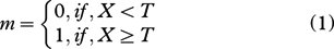
Generally, snowmelt detection methods involve the problem of classifying melt signals (X) for dry snow and wet snow. The melt signal is some quantification of dry snow and wet snow. For example, in the XPGR method, the XPGR value is used as melt signal to indicate wet snow or dry snow, and the critical value (Liu et al. 2005) is used as melt signal in wavelet transformation-based edge detection approach. Let m represent the melt detection, with m=1 indicating melt and m=0 indicating non-melt:
The classification precision (determined by the threshold T) of dry snow and wet snow will directly influence the accuracy of the calculated results of ice-sheet snowmelt distribution and is therefore formulated as a determination of the optimal threshold of dry snow and wet snow. If the melt signal X of dry snow and wet snow is considered as a random variable, the optimal threshold can be determined by using statistical inference based on the statistical characteristics of the melt signal of dry snow and wet snow. Let h(Xl), Xl=0,1,…,L−1 be the histogram of melt signal samples of dry snow and wet snow, where L stands for the number of the maximum melt signal. The histogram h(Xl) can be considered an approximation of the actual probability density function  of the mixture population describing the wet snow and dry snow. In the Kittler-Illingworth (KI) threshold selection criterion (Kittler & Illingworth 1986), the selection of an appropriate decision threshold T∈{0,1,…,L−1} is based on the optimization of the criterion function:
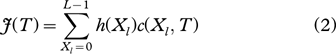
The function c(Xl,T) over the histogram h(Xl) is a cost function, which measures the cost of classifying snow by comparing their melt signal with the threshold T. The optimal threshold that minimizes the classification error is the one that minimizes the following cost function:

Determining cost function depends on the probability density function (pdf) of melt signal of dry snow and wet snow. Because different detection methods use different melt signals, the pdfs of melt signals of different methods is likely to be different. For this reason, we considered a model that should be adaptable to the pdfs of different melt signals; that is, it should be capable of spanning a large variety of statistical behaviours. Moreover, for easy implementation during regular operation, it should not require the estimation of an excessively large number of parameters. Among the possible models, the GG distribution is a particularly attractive candidate. The analytical expression of the GG distribution considered in our approach for modelling the two class-conditional pdfs is given by (Sharifi & Leon-Garcia 1995; Niehsen 1999):

where the positive constants ai and bi are given by:
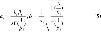
The terms mi,
 and βi are the mean, the variance and the shape parameters of the distribution, respectively, and Γ(·) is the well-known Gamma function. We can see from Eqn. 5 that the GG model requires the estimation of only three parameters, which are mi,
and βi. The shape parameter βi, in the GG model, tunes the decay rate of the density function. When βi
=2, the GG density function is actually the Gaussian density function, and βi=1, it is the Laplacian density function. Moreover, in the limit case βi→0 or βi→∞, it approaches an impulsive function or uniform distribution, respectively. Thus, the GG model can adapt to a large class of statistical distributions.
and βi are the mean, the variance and the shape parameters of the distribution, respectively, and Γ(·) is the well-known Gamma function. We can see from Eqn. 5 that the GG model requires the estimation of only three parameters, which are mi,
and βi. The shape parameter βi, in the GG model, tunes the decay rate of the density function. When βi
=2, the GG density function is actually the Gaussian density function, and βi=1, it is the Laplacian density function. Moreover, in the limit case βi→0 or βi→∞, it approaches an impulsive function or uniform distribution, respectively. Thus, the GG model can adapt to a large class of statistical distributions.
Under the GG distribution assumption, it can be proved that the cost function is optimized as follows (see the Supplementary File):
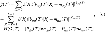
where:
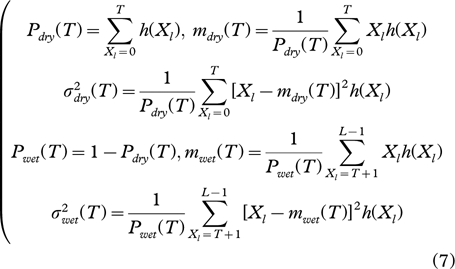
Pdry(T) and Pwet(T) are the prior probabilities; mdry(T) and mwet(T) are the means;  and
and  are the variances; βdry(T) and βwet(T) are the shape parameters of the distribution. These parameters are all associated with the dry snow and wet snow samples, respectively, for a given value of the threshold T. H(Ω,T) stands for the entropy associated with the binary set of classes Ω={ωdry, ωwet1}. For the steps to estimate ai, bi, βi, please refer to Sharifi & Leon-Garcia (1995).
As shown above, the advantages of the GG model method are: it requires less manual input parameters (the parameters are computed automatically); the classification result is unique (namely, the threshold is unique); and it is capable of spanning a large variety of statistical behaviours.
The melt signal adaptation method can be applicable to many different melt signals in many different snowmelt detection methods, for example the XPGR value in XPGR method, the normalized gradient ratio (GR) value in GR method  the critical value in the ice-sheet snowmelt detection method based on wavelet transformation, the melt signal X in α-based Tb melt detection method
 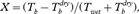 and so on.
Here, we only apply the method to the existing XPGR and wavelet transformation-based ice-sheet snowmelt detection methods. Further work will focus on the GR method, the α-based method and other methods.
Implementing the XPGR ice-sheet snowmelt detection method
The XPGR method proposed by Abdalati & Steffen (1995) mainly utilized the different response of two frequencies (19 GHz and 37 GHz) and two polarizations (horizontal and vertical) on ice sheets to detect snowmelt. The advantage of this method is that the response differences of frequency and polarization to emissivity and moisture contents were used which clearly showed snowmelt information and that the model was stable. The XPGR equation is:
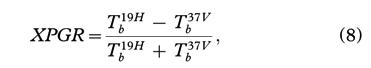
where  is the microwave brightness temperature at the 19-GHz horizontally (19H) polarized channel and
  is the microwave brightness temperature at the 37-GHz vertically (37V) polarized channel.
Figure 2 shows the XPGR long time series change derived from SMMR and SSM/I data sets from 1978 to 2010 at the Wilkins Ice Shelf area in Antarctica, which experienced melting every year. By sampling XPGR values both in the summer season (November, January and February) and other seasons, we analysed the statistical characteristics of the XPGR values of wet and dry pixels. Figure 3 shows the histogram of XPGR values. The distribution characteristics of XPGR values of dry snow generally have a low mean value whereas for wet snow the mean values are generally higher. As we can see in Fig. 3, the XPGR values are divided into two dominant categories with a valley between them: to the left are low values that indicate the distribution characteristics of dry snow; to the right are higher values representing wet snow. To model a bimodal histogram of XPGR values, we can consider it as a mixture of two GG models. Then, we computationally obtain an optimal threshold value for separating wet pixels from dry pixels by applying the melt signal adaptation method. The XPGR optimal threshold calculated from the method is −0.0239 (see Figs. 3, 4). Figure 4 shows that the optimal XPGR value corresponds to sharply changed regions, namely, it corresponds to time points when snow changed from dry to wet or from wet to frozen. We propose a modified XPGR detection method, based on this. Figure 5 is a flowchart of the modified XPGR detection method.

Fig. 2
Cross-gradient polarization ratio (XPGR) values at the Wilkins Ice Shelf area (from 1978 to 2010).

Fig. 3
Cross-gradient polarization ratio (XPGR) histogram and optimal threshold at the Wilkins Ice Shelf area (from 1978 to 2010). The red asterisk is the unsupervised XPGR threshold (−0.0293) obtained by the melt signal adaptation method.

Fig. 4
Segmentation line of the optimal threshold at the Wilkins Ice Shelf area (from 1978 to 2010). The red line is the unsupervised Cross-gradient polarization ratio (XPGR) threshold (−0.0293) obtained by the melt signal adaptation method.

Fig. 5
Flowchart of modified cross-gradient polarization ratio (XPGR) detection method. Scanning Multichannel Microwave Radiometer is abbreviated to SMMR and Special Sensor Microwave/Imager to SSM/I.
Implementing the ice-sheet snowmelt detection method based on wavelet transformation
Ice-sheet snowmelt detection using a wavelet transformation-based method is based on the strong and significant edges in the brightness temperature (Tb) time series curve that signify snow melting and refreezing events (Liu et al. 2005). The basic steps are as follows. First, the time series brightness temperature values of each pixel are decomposed into multi-scale components through a wavelet transform. Second, the local extrema of the wavelet transform modulus (modulus extrema), which indicate the strength of the edges caused by sharp transitions and the time when the sharp variations occur, are tracked and analysed across scales. Third, for each pixel, a critical value as a melt signal to differentiate the sharp transition induced by melting and refreezing processes from other transitions caused by non-melt processes is determined by variance analysis. Then, based on critical values of samples of wet pixels and dry pixels, a bimodal Gaussian (BG) model fitting technique is used to statistically determine an optimal edge threshold to classify wet snow and dry snow. Finally, based on the principle of spatial autocorrelation, a spatial neighbourhood operator is used to detect and correct possible errors brought about by the strong noise of data pixels. This method can determine not only whether an area experienced melt, but also when an area experienced melt by detecting and tracking strong and significant edges in the brightness temperature time series curve.
Liu et al. (2005) used the BG model fitting to determine the optimal threshold. As stated in an earlier section in this article, the GG model is also adaptable to the BG model of melt signal for the wavelet-based method. It is therefore possible to apply the melt signal adaptation method to the existing ice-sheet snowmelt detection method based on wavelet transformation. Through selection of the samples of wet and dry snow in Antarctica based on the metrics of Liu et al. (2005), sampling both wet pixels that experienced melting and dry pixels that remained dry, we use the GG models to determine the thresholds of dry snow and wet snow based on the Antarctic SMMR 18-GHz horizontal polarization channel data and the SSM/I and SSMIS 19-GHz horizontal channel data from 1978 to 2010.
Figure 6 shows the optimal threshold—10.30—derived from the melt signal adaptation method. Using this, we propose a modified ice-sheet snowmelt detection method based on wavelet transformation (Fig. 7).

Fig. 6
Two optimal thresholds obtained from a bimodal Gaussian distribution model (BG) and a generalized Gaussian model (GG).

Fig. 7
Flowchart of the modified ice-sheet snowmelt detection method based on wavelet transformation. Scanning Multichannel Microwave Radiometer is abbreviated to SMMR and Special Sensor Microwave/Imager to SSM/I.
Result analysis and validation
Comparison analysis
The difference between the modified XPGR detection method and the XPGR method lies in the method in which the threshold is determined. The XPGR method uses in situ measurements to determine the threshold. The modified XPGR method uses the GG model to automatically seek an optimal threshold. Therefore, the modified XPGR method is solely dependent on the XPGR value. To analyse and compare the results of the method proposed by Abdalati & Steffen (1997), SSM/I data from 1988 to 2000 at the same experimental area (Swiss Camp, Greenland, 69°34′N, 49°17′W, 1150 m a.s.l.) is used.
Figure 8 shows the XPGR threshold determination respectively based on Abdalati & Steffen’s (1997) method and the modified method in the Greenland study area. It is evident that the difference between the XPGR threshold obtained by Abdalati & Steffen (1997) and the unsupervised XPGR threshold is very small.

Fig. 8
The threshold determination based on cross-gradient polarization ratio (XPGR) value in the Greenland study area. The solid blue line represents the XPGR values from 1988 to 1995, the red line is the XPGR threshold (−0.0158) obtained by Abdalati & Steffen’s (1997) method, and the light blue line is the unsupervised XPGR threshold (−0.0152).
Figure 9 shows ice-sheet snowmelt distribution drawn from the two methods on 2 August 1996. The white indicates melt area, and grey indicates the non-melt area or bare rock area. The results of the two methods are almost the same, with only small differences seen. Near the AWS at Swiss Camp, the modified XPGR method did not detect melting on snow surface. Meanwhile, the maximum temperature measured by this station was −2.59°C (temperature measured at 1 m above the snow surface) on 2 August 1996, which indicates that it is highly possible that no melting occurred around this area. This result supports the accuracy of the proposed method.

Fig. 9
Ice-sheet snowmelt distribution of the modified cross-gradient polarization ratio (XPGR) detection method and the XPGR method on 2 August 1996: (a) the result of the XPGR method; (b) the result of the modified XPGR method.
Analysis and comparison of the modified and original wavelet transformation detection method results are based on the Antarctic SSM/I data from 1978 to 2010. Figure 7 is a flowchart of the ice-sheet snowmelt detection method based on wavelet transformation (Liu et al. 2005). The difference between the modified wavelet transformation detection method and the original method is that the original uses the BG model to determine optimal threshold, whereas the modified wavelet transformation detection method uses the GG model-based method to seek an optimal threshold. In Fig. 6, we can see that the optimal threshold value for the optimal threshold derived from the BG method l is 10.28 whereas that for the modified method is 10.30.
Figure 10 shows the ice-sheet snowmelt distributions obtained from the modified wavelet transformation detection method and the original method during 2007–08. The two results are similar, but the result obtained from the BG distribution model shows that there is some inland melting in Antarctica, which is unlikely. In contrast, the GG model automatic threshold segmentation indicates no such melting. Figure 11 shows melt onset, melt end and melt duration distribution obtained from the modified wavelet transformation detection method in Antarctica during 2007–08.

Fig. 10
Ice-sheet snowmelt distribution during 2007–08 derived from the two optimal thresholds: (a) the bimodal Gaussian distribution model optimal threshold; (b) the generalized Gaussian model automatic threshold.

Fig. 11
Ice-sheet snowmelt detection results obtained from the modified wavelet transformation method in Antarctica, 2007–08: (a) melt onset; (b) melt end; (c) melt duration.
This comparison shows that the optimal threshold based on the GG model is almost the same as those based on the BG model. However, the melt signal adaptation method increases threshold determination efficiency, has higher accuracy and is independent of estimation and initial value.
Validation using in situ data
In addition to comparing the results of the modified and original methods, we have performed quantitative validations on the effectiveness and precision of the modified ice-sheet snowmelt detection method.
We use in situ data to validate the daily snowmelt detection results of each method. In general, surface melting occurrence spatially corresponds to the spatial pattern of temperature. Therefore, we validate the snowmelt detection results derived from two methods with the corresponding surface air temperature acquired by AWSs. An AWS cannot cover the same area observed by large-scale remote sensing and can therefore not completely reflect large-scale climate. However, to minimize the influence of the environment, we choose AWSs in those areas where the spatial gradients are relatively simple because the temperature data collected on these stations can reflect average temperature of large areas to some degree. Based on the Radarsat Antarctic Mapping Project Digital Elevation Model, we use the 1-km data to calculate the minimum height, maximum height and standard deviation of height in the 625 km2 area around the AWS. We use those parameters as a standard of evaluation of spatial complexity. We choose the AWS in the area where the standard deviation of height and difference between the extreme values of height and elevation of AWS are smallest.
Because of the limited temperature records and strong fluctuations in surface melt on the Ross Ice Shelf, on the Ronne-Filchner Ice Shelf and in Marie Byrd Land AWSs were not chosen in those regions. The AWSs on Butler Island, at Bonaparte Point, on Larsen Shelf and at Amery G3 were chosen (Table 2).
Table 2 Automatic weather stations.
| Station name |
Latitude/longitude |
Elev. |
Dates |
Days |
Min. |
Max. |
SD |
| Larsen Ice Shelf |
66.90S/60.60W |
50 m |
07/02/83–01/01/86 |
2390 |
36.46 m |
49.78 m |
1.6874 |
| – |
66.97S/60.55W |
– |
01/01/86–01/02/99 |
– |
– |
– |
– |
| |
66.949S/60.897W |
|
01/02/99–02/01/04 |
|
|
|
|
| |
67.012S/61.550W |
|
02/01/04–01/01/07 |
|
|
|
|
| |
67.012S/61.550W |
|
01/01/07– |
|
|
|
|
| Butler Island |
72.20S/60.34W |
91 m |
01/03/86–25/01/89 |
2449 |
−14.80 m |
95.36 m |
16.83 |
| – |
72.21S/60.16W |
– |
25/01/89–11/01/97 |
– |
– |
– |
– |
| |
72.21S/60.17W |
|
11/01/97–11/01/00 |
|
|
|
|
| |
72.207S/60.160W |
|
11/01/00–22/12/03 |
|
|
|
|
| |
72.206S/60.170W |
|
02/02/05–02/02/11 |
|
|
|
|
| |
72.206S/60.170W |
|
02/02/11– |
|
|
|
|
| Bonaparte Point |
64.78S/63.06W |
8 m |
05/01/92–09/03/94 |
1761 |
−35.10 m |
311.72 m |
77.97 |
| – |
64.78S/63.07W |
– |
09/03/94–23/12/96 |
– |
– |
– |
– |
| |
64.778S/63.067W |
|
23/12/96–14/03/08 |
|
|
|
|
| |
64.778S/63.067W |
|
14/03/08–20/11/09 |
|
|
|
|
| |
64.778S/63.067W |
|
20/11/09– |
|
|
|
|
| Amery G3 |
70°53′31′′S/69°52′21′′E |
84 m |
1999– |
1931 |
95.20 m |
104.08 m |
1.84 |
The daily mean air temperature data together with the corresponding daily detection results of each modified snowmelt detection method were used to quantitatively validate the snowmelt detection results of each method. For processing the AWS data, we chose the daily mean air temperature data from the summer months (November–March) in Antarctica. The total number of days N (i.e., the total number of daily mean air temperature data) chosen in each AWS can be seen in Table 2. The daily mean air temperature data are made up of the mean of three daily maximum air temperatures; a daily mean air temperature data above 0°C is regarded as snowmelt occurrence. A melt day is the day with daily mean air temperature data above 0°C and a non-melt day is the day whose daily mean air temperature data is below 0°C. Once the corresponding daily detection results have been obtained by using the snowmelt detection method, the following defined quantities (Celik 2010) are computed for comparing the daily detection results against the corresponding daily mean air temperature data:
- True positives (TP): the number of melt days that were correctly detected, and PTP=TP/N.
- False positives (FP): the number of non-melt days that were incorrectly detected as “melt” (also known as false alarms), and PFP=TP/N.
- True negatives (TN): the number of non-melt days that were correctly detected, and PTP=TP/N.
- False negatives (FN): the number of melt days that were incorrectly detected as “non-melt” (also known as miss detections), and PFP=TP/N.
Based on these four quantities, three assessment indices are proposed to evaluate the snowmelt detection result of the proposed method. The three assessment indices are as follows: Correct Detection Rate (CDR), Priori True Positives Rate (Priori TPR) and Posterior True Positives Rate (Posterior TPR). CDR is the ratio between the number of correctly detection results and the total number of detection results (or the total number of temperature data); Priori TPR is the ratio between the number of correctly detected “melt” results and the number of temperature data above 0°C; Posterior TPR is the ratio between the number of correctly detected “melt” results and the number of detected “melt” results:


The statistical analysis results are shown in Table 3. For CDR, two methods have relatively high probabilities in several areas around the AWSs. The percentages of CDR exceed 65%, except for the XPGR methods in the area around the Bonaparte Point AWS. The CDR indicated that the improvements on two snowmelt detections are effective.
Table 3 Quantitative snowmelt detection results (in %), applying two methods in four areas.
| Automatic weather station |
Snowmelt detection method |
PTPa
|
PFPb |
PTNc |
PFNd |
CDRe
|
Priori TPRf
|
Posterior TPRg
|
| Bonaparte Point |
Wavelet |
55.03 |
4.49 |
12.66 |
27.83 |
67.69 |
66.42 |
92.46 |
| |
XPGRh
|
32.14 |
3.35 |
13.80 |
50.71 |
45.94 |
38.79 |
90.56 |
| Butler Island |
Wavelet |
6.7 |
15.03 |
71.87 |
6.41 |
78.56 |
51.09 |
30.83 |
| |
XPGR |
4.08 |
14.56 |
72.02 |
9.34 |
76.09 |
30.38 |
21.87 |
| Larsen Ice Shelf |
Wavelet |
22.51 |
13.14 |
51.38 |
12.97 |
73.89 |
63.44 |
63.15 |
| |
XPGR |
26.16 |
20.81 |
45.59 |
7.44 |
71.75 |
77.86 |
55.70 |
| Amery G3 |
Wavelet |
4.97 |
9.01 |
83.43 |
2.59 |
88.40 |
65.75 |
35.56 |
| |
XPGR |
5.58 |
20.42 |
71.90 |
2.09 |
77.49 |
72.73 |
21.48 |
| aThe number of melt days that were correctly detected. |
| bThe number of non-melt days that were incorrectly detected as “melt” days. |
| cThe number of non-melt days that were correctly detected. |
| dThe number of melt days that were incorrectly detected as “non-melt” days. |
| eCorrect detection rate, the ratio between the number of correct detection results and the total number of detection results. |
| fPriori true positives rate, the ratio between the number of correctly detected “melt” results and the number of temperature data above 0°C. |
| gPosterior true positives rate, the ratio between the number of correctly detected “melt” results and the number of detected “melt” results. |
| hCross-gradient polarization ratio. |
However, we were primarily concerned with Priori TPR and Posterior TPR. Although the comparative statistics with in situ data were collected at the Bonaparte Point AWS and the Larsen Ice Shelf AWS, the result values of both methods show relatively high probabilities, except the XPGR methods in the area around the Bonaparte Point AWS. Moreover, the Posterior TPR of both methods are over 90%. For the Amery G3 AWS, the Priori TPR of both methods are over 65%; however, the Posterior TPR show relatively low probabilities. For the Butler Island AWS, both methods have low Priori TPR and low Posterior TPR. This is because the Butler Island AWS is very close to the seaside, so it does not reflect the average temperature of a large adjacent inland area.
Using temperature data to validate the snowmelt detection results of the modified XPGR detection method and the modified wavelet transformation-based method shows that they have relatively high precision.
Conclusions
This paper reports the results of an ice-sheet snowmelt detection study using microwave radiometer data sets. We proposed a melt signal adaptation method to automate melt signal detection, based on a GG model, for a variety of melt signals derived from two different ice-sheet snowmelt detection methods. We proposed a modified XPGR snowmelt method and a modified snowmelt detection method based on wavelet transformation edge detection. By comparing the two methods and validating them with temperature data from AWSs, we found that the methods not only ensure computational efficiency, practicability and operability due to independence from in situ measurement, but also—to some extent—improve ice-sheet snowmelt detection accuracy over the original methods. The two proposed methods can be used to efficaciously determine the threshold for various snowmelt detection methods in different ice sheets. Most importantly, the method can be adapted to different kinds of melt information. The signal melt adaptation method provides methodological support for an ice-sheet snowmelt monitoring system.
Acknowledgements
This research was supported by the National Natural Science Foundation of China (General Programme, no. 41076129) and the National High-tech R&D Program of China (Programme 863, no. 2008AA121702).
References
Abdalati
W. & Steffen
K. 1995.
Passive microwave-derived snow melt regions on the Greenland Ice Sheet. Geophysical Research Letters 22,
787–790.
Publisher Full Text
Abdalati
W. & Steffen
K. 1997.
Snowmelt on the Greenland Ice Sheet as derived from passive microwave satellite data. Journal of Climate 10,
165–175.
Abdalati
W., Steffen
K., Otto
C. & Jezek
K.C. 1995.
Comparison of brightness temperatures from SSMI instruments on the DMSP F8 and F11 satellites for Antarctica and the Greenland Ice Sheet. International Journal of Remote Sensing 16,
1223–1229.
Publisher Full Text
Aschraft
I.S. & Long
D.G. 2006.
Comparison of methods for melt detection over Greenland using active and passive microwave measurements. International Journal of Remote Sensing 27,
2469–2488.
Publisher Full Text
Celik
T. 2010.
Image change detection using Gaussian mixture model and genetic algorithm. Journal of Visual Communication and Image Representation 21,
965–974.
Publisher Full Text
Huybrechts
P. 2004.
Antarctica: modelling.
In J.L. Bamber & A.J. Payne (eds.): Mass balance of the cryosphere: observations and modelling of contemporary and future changes. Pp. 491–523. Cambridge: Cambridge University Press.
Jezek
K.C., Merry
C., Cavalieri
D., Grace
S., Bedner
J., Wilson
D. & Lampkin
D. 1991. Comparison between SMMR and SSM/I passive microwave data collected over the Antarctic ice sheet. Byrd Polar Research Center Technical Report 91–03. Columbus: Ohio State University.
Joshi
M., Merry
C.J., Jezek
K.C. & Bolzan
J.F. 2001.
An edge detection technique to estimate melt duration, season and melt extent on the Greenland Ice Sheet using passive microwave data. Geophysical Research Letters 28,
3497–3500.
Publisher Full Text
Kittler
J. & Illingworth
J. 1986.
Minimum error thresholding. Pattern Recognition 19,
41–47.
Publisher Full Text
Liu
H., Wang
L. & Jezek
K. 2005.
Wavelet-transform based edge detection approach to derivation of snowmelt onset, end and duration from satellite passive microwave measurements. International Journal of Remote Sensing 26,
4639–4660.
Publisher Full Text
Matzler
C. & Wiesmann
A. 1999.
Extension of the microwave emission model of layered snowpacks to coarse-grained snow. Remote Sensing of Environment 70,
307–316.
Publisher Full Text
Mote
T.L., Anderson
M.R., Kuivinen
K.C. & Rowe
CM. 1993.
Passive microwave-derived spatial and temporal variations of summer melt on the Greenland Ice Sheet. Annals of Glaciology 17,
233–238.
Niehsen
W. 1999.
Generalized Gaussian modeling of correlated signal sources. IEEE Transactions on Signal Processing 47,
217–219.
Publisher Full Text
Ramage
J.M. & Isacks
B.L. 2003.
Interannual variations of snowmelt and refreeze timing in southeast Alaskan iceshields using SSM/I diurnal amplitude variations. Journal of Glaciology 49,
102–116.
Publisher Full Text
Sharifi
K. & Leon-Garcia
A. 1995.
Estimation of shape parameter for generalized Gaussian distributions in subband decomposition of video. IEEE Transactions on Circuits and Systems for Video Technology 5,
52–56.
Publisher Full Text
Steffen
K., Abdalati
W. & Stroeve
J. 1993.
Climate sensitivity studies of the Greenland Ice Sheet using satellite AVHRR, SMMR, SSM/I and in situ data. Meteorology and Atmospheric Physics 51,
239–258.
Publisher Full Text
Takala
M., Pulliainen
J., Huttunen
M. & Hallikainen
M. 2003. Estimation of the beginning of snow melt period using SSM/I data. Geoscience and Remote Sensing Symposium, 2003. IGARSS ’03. Proceedings. 2003 IEEE International 4. Pp. 2841–2843. New York: Institute of Electrical and Electronics Engineers.
Takala
M., Pulliainen
J., Huttunen
M. & Hallikainen
M. 2008.
Detecting the onset of snow-melt using SSM/I data and the self-organizing map. International Journal of Remote Sensing 29,
755–766.
Publisher Full Text
Takala
M., Pulliainen
J., Metsämäki
S.J. & Koskinen
J.T. 2009.
Detection of snowmelt using spaceborne microwave radiometer data in Eurasia from 1979 to 2007. IEEE Transactions on Geoscience and Remote Sensing 47,
2996–3007.
Publisher Full Text
Tedesco
M. 2009.
Assessment and development of snowmelt retrieval algorithms over Antarctica from K-band space borne brightness temperature (1979–2008). Remote Sensing of Environment 113,
979–997.
Publisher Full Text
Tedesco
M., Abdalati
W. & Zwally
H.J. 2007. Persistent surface snowmelt over Antarctica (1987–2006) from 19.35 GHz brightness temperatures. Geophysical Research Letters
34, L18504, doi: 10.1029/2007GL031199.
Publisher Full Text
Torinesi
O., Fily
M. & Genthon
C. 2003.
Interannual variability and trend of the Antarctic summer melting period from 20 years of spaceborne microwave data. Journal of Climate 16,
1047–1060.
Ulaby
F.T., Moore
R.K. & Fung
A. 1986. Microwave remote sensing: active and passive. Vol. 3. From theory to application. Norwood, MA: Artech House.
Warrick
R.A. & Oerlemans
H. 1990.
Sea level rise.
In J.T. Houghten et al. (eds.): Climate change: the IPCC scientific assessment. Pp. 257–282. New York: Cambridge University Press.
Zwally
H.J. & Fiegles
S. 1994.
Extent and duration of Antarctic surface melting. Journal of Glaciology 40,
463–476.
Zwally
H.J. & Gloersen
P. 1977.
Passive microwave images of the polar regions and research applications. Polar Record 18,
431–450.
Publisher Full Text